NumPy API function notes

Some notes on functions I picked up while learning.

The where function

The official docs.

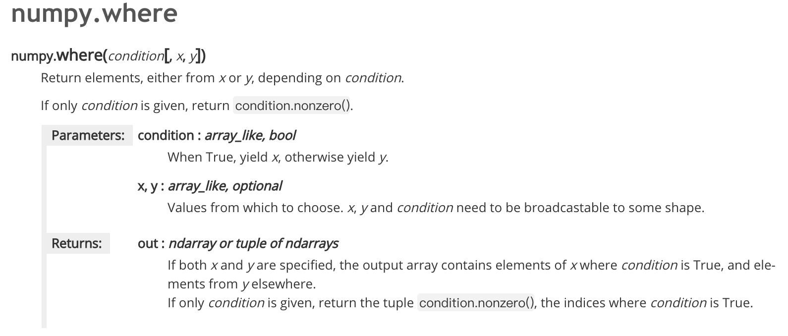
The docs alone didn’t quite click for me.

numpy.where() has two forms:

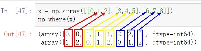
1. np.where(condition, x, y) — where the condition holds, output x; otherwise output y.
2. np.where(condition) — with only a condition and no x/y, it returns the coordinates of the elements that satisfy the condition (i.e. the non-zero ones; equivalent to numpy.nonzero). The coordinates come back as a tuple: an N-dimensional input yields a tuple of N arrays, each holding one dimension’s coordinates.

A Zhihu answer illustrates it clearly:

The first form:

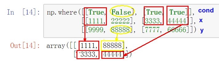
and likewise:

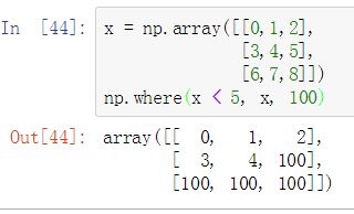
The second form — only a condition, returning the coordinates of the satisfying (non-zero) elements. Each column is one element’s full coordinate:

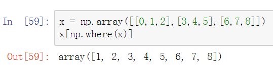
so:

numpy.random.multinomial

Official docs.

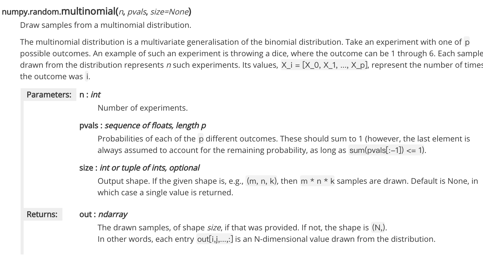
This is NumPy’s binomial sampler. The binomial distribution is:

$$P(N)=\begin{pmatrix}n \\ N \end{pmatrix}p^N(1-p)^{n-N}$$

The signature:

numpy.random.RandomState.binomial(n, p, size=None)

It samples from a binomial distribution; size is the number of samples, n and p match $n,p$ in the formula, and the return value is the number of successes (i.e. $N$). For example, with 3 coins each flipped once, what’s the probability all three come up heads?

Basic probability gives:

$$P=\begin{pmatrix}n \\ N\end{pmatrix}p^N(1-p)^{n-N}=\begin{pmatrix}3 \\ 3\end{pmatrix}0.5^3(1-0.5)^0=0.5^3 = 0.125$$

Estimating it with the sampler means running enough trials and taking the frequency of “all heads” as the probability:

Element-wise (*) vs. matrix (.dot) multiplication

import numpy
a = numpy.array([[1,2],
                 [3,4]])
b = numpy.array([[5,6],
                 [7,8]])

Results:

a*b
>>>array([[ 5, 12],
          [21, 32]])

a.dot(b)
>>>array([[19, 22],
          [43, 50]])

numpy.dot(a,b)
>>>array([[19, 22],
          [43, 50]])

numpy.dot(b,a)
>>>array([[23, 34],
          [31, 46]])

* multiplies matrices element-wise (sizes must match). .dot is the matrix product, following the usual rules of matrix multiplication.

meshgrid()

This returns coordinate matrices from coordinate vectors — handy in many places, e.g. building the data grid for a contour plot.

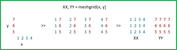
meshgrid() takes two 1-D vectors and produces a coordinate matrix.

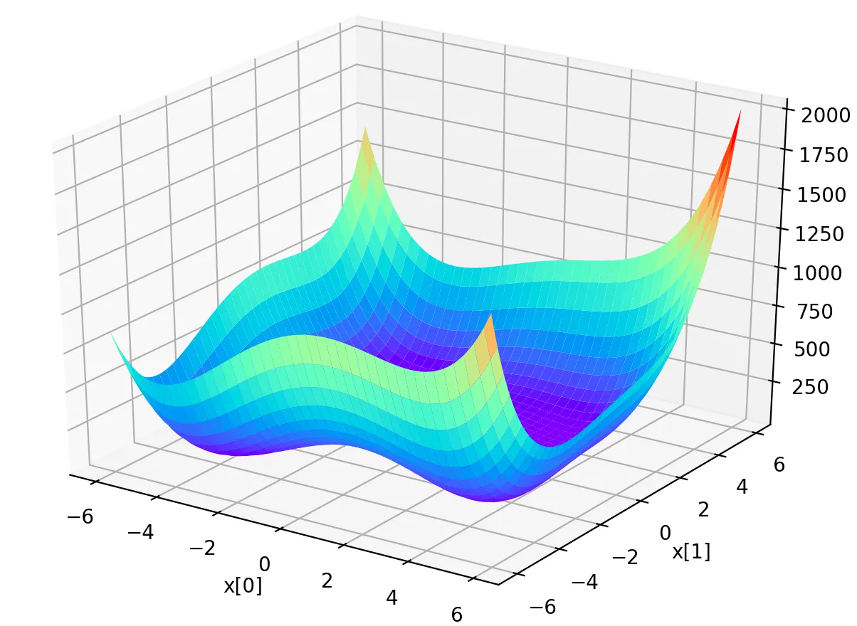
For instance, when visualizing himmelblau:

import numpy as np
from mpl_toolkits.mplot3d import Axes3D
import matplotlib.pyplot as plt

def himmelblau(x):
    return (x[0] ** 2 + x[1] - 11) ** 2 + (x[0] + x[1] ** 2 - 7) ** 2


x = np.arange(-6, 6, 0.1)
y = np.arange(-6, 6, 0.1)
X, Y = np.meshgrid(x, y)
Z = himmelblau([X, Y])

fig = plt.figure()
ax = Axes3D(fig)
ax.plot_surface(X, Y, Z, cmap='rainbow')
ax.set_xlabel('x[0]')
ax.set_ylabel('x[1]')
plt.show()

The result: